Tutorial

In this tutorial, we will:

• Create a hybrid simulation between an Agent-based model, defined in Agents.jl, and an ODE system defined through DifferentialEquations.jl.
• Introduce Sirens Components for Agents.jl and DifferentialEquations.jl.
• Demonstrate how these Components can be connected together through Connectors.
• Solve the hybrid model.
• Visualise the results of the simulation.

This example will include a group of birds, flocking around some food at a single moving point, where the motion of the moving point is governed by an ODE system.

Components

To begin, we need to define our components. These will be an ODE model component for the movement of the food, and an Agent-based model component for the birds.

Differential Equations Components

To define the ODE model, let's have a look at how to define an ODE Component.

DEComponent(model::DiffEqBase.AbstractDEProblem, alg;
            name::String="DE", timestep::Float64=1.0, intkwargs::NamedTuple=(;),
            state_names::Dict{String,Any}=Dict{String,Any}())
DEComponent(model::DiffEqBase.AbstractDEProblem; kwargs...)

function f!(du, u, p, t)
    du[1] = -u[1]
end
prob = ODEProblem(f!, [1.0], (0.0, 10.0))
comp = DEComponent(prob, Tsit5(); name="ode_comp",
                   state_names=Dict("x" => 1))

We see that we need to define an ODEProblem to use in the component, so let's create one.

using OrdinaryDiffEq
function food!(du, u, p, t)
    x, y = u
    d = 10.0
    mu = 1.3
    tau = 30.0
    du[1] = (y - 50)/tau
    du[2] = (mu * (1 - (x-50)^2/d^2)*(y-50) - (x-50))/tau
end
u0 = [40.0, 40.0]
tspan = (0.0, 500.0)
prob = ODEProblem(food!, u0, tspan)

Next, we want to wrap this ODEProblem inside an DEComponent. For this, we will need to define the state_names field, and should generally provide a value for the name field (since component names in a hybrid simulation should be unique).

using Sirens
comp1 = DEComponent(prob, Rodas5P();
    name="food", state_names=Dict("x" => 1, "y" => 2),
)

Agents.jl Components

Now that we have created our DEComponent, we can move on to the AgentsComponent, so let's have a look at its documentation.

AgentsComponent(model::StandardABM; name="Agents Component",
                state_names=Dict{String,Any}(), timestep::Real=1.0)

comp = AgentsComponent(model;
    name="abm_comp",
    state_names=Dict("x" => :pos_x, "y" => :pos_y))

We can see that, again, we need to define the model (this time a StandardABM from Agents.jl), a name and a state_names.

using Agents, Random, LinearAlgebra
@agent struct Bird(ContinuousAgent{2, Float64})
    const speed::Float64
    const visual_distance::Float64
    const turn_speed::Float64
end

function initialize_model(;
        n_birds = 100,
        speed = 1.0,
        visual_distance = 15.0,
        turn_speed = 0.04,
        extent = (100, 100),
        seed = 0
)
    space2d = ContinuousSpace(extent)
    rng = Random.MersenneTwister(seed)

    props = Dict(:food_x => rand() * extent[1],
        :food_y => rand()*extent[2])

    model = StandardABM(
        Bird, space2d; rng, agent_step!, container = Vector, properties = props)
    for _ in 1:n_birds
        vel = rand(abmrng(model), SVector{2}) * 2 .- 1
        add_agent!(
            model,
            vel,
            speed,
            visual_distance,
            turn_speed
        )
    end
    return model
end

function agent_step!(bird, model)
    heading = get_direction(bird.pos, (model.food_x, model.food_y), model)

    if sum(heading .^ 2) < bird.visual_distance^2
        # Bird can see food so should head towards food
        bird.vel += bird.turn_speed * heading
    else
        # Bird can't see food so should turn towards nearest bird
        nearest_bird = nearest_neighbor(bird, model, bird.visual_distance)
        if !isnothing(nearest_bird)
            heading = get_direction(bird.pos, nearest_bird.pos, model)
        else
            heading = (0, 0)
        end
        bird.vel += bird.turn_speed * (heading .+ randn(abmrng(model), SVector{2}))
    end
    bird.vel /= norm(bird.vel)

    return move_agent!(bird, model, bird.speed)
end

model = initialize_model()

comp2 = AgentsComponent(model;
    name = "birds", state_names = Dict("x" => :food_x, "y" => :food_y)
)

AgentsComponent{StandardABM{ContinuousSpace{2, true, Float64, typeof(Agents.no_vel_update)}, Main.Bird, Vector{Main.Bird}, Tuple{DataType}, typeof(Main.agent_step!), typeof(dummystep), typeof(Agents.Schedulers.fastest), Dict{Symbol, Float64}, Random.MersenneTwister}, String, Dict{String, Symbol}, Int64}(StandardABM with 100 agents of type Bird
 agents container: Vector
 space: periodic continuous space with [100.0, 100.0] extent and spacing=5.0
 scheduler: fastest
 properties: food_y, food_x, "birds", Dict("x" => :food_x, "y" => :food_y), 1)

Connections

We can now set up the connections between the variables in the two components.

Connector <: AbstractConnector

The format for specifying a ConnectedVariable is given in Sirens Interface, but in its simplest form, it is a string containing a component name and a variable/state name.

conn1 = Connector(inputs=["food.x"], outputs=["birds.x"])
conn2 = Connector(inputs=["food.y"], outputs=["birds.y"])

Connector{Tuple{ConnectedVariable{SubString{String}, SubString{String}, Nothing, Nothing}}, Tuple{ConnectedVariable{SubString{String}, SubString{String}, Nothing, Nothing}}}((ConnectedVariable{SubString{String}, SubString{String}, Nothing, Nothing}("food", "y", nothing, nothing),), (ConnectedVariable{SubString{String}, SubString{String}, Nothing, Nothing}("birds", "y", nothing, nothing),), nothing)

Solving the hybrid model

To create the hybrid model, we need to create a SirenProblem. We can then solve this using the CommonSolve interface.

SirenProblem <: AbstractSirenProblem
SirenProblem(components, connectors, tspan, timescales=ones(length(components)))
SirenProblem(;
    components::Union{Tuple, Vector},
    connectors::Union{Tuple, Vector},
    tspan::Tuple{Float64, Float64},
    timescales::Vector{Float64}=ones(length(components)))

sp = SirenProblem(components=[comp1, comp2], connectors=[conn1, conn2], tspan=tspan)
alg = MinimumTimeStepper()
sol = solve(sp, alg)

SirenSolution{Vector{Float64}, Sirens.SirenSolutionData{NTuple{4, ConnectedVariable{String, String, Nothing, Nothing}}, NTuple{4, Vector{Float64}}}}([0.0, 1.0, 2.0, 3.0, 4.0, 5.0, 6.0, 7.0, 8.0, 9.0  …  491.0, 492.0, 493.0, 494.0, 495.0, 496.0, 497.0, 498.0, 499.0, 500.0], Sirens.SirenSolutionData{NTuple{4, ConnectedVariable{String, String, Nothing, Nothing}}, NTuple{4, Vector{Float64}}}((ConnectedVariable{String, String, Nothing, Nothing}("food", "x", nothing, nothing), [40.0, 39.67244109021822, 39.357277117242305, 39.055703030964466, 38.76880195388508, 38.49753160657571, 38.242714170867806, 38.00502984480508, 37.785014155017464, 37.58305891009925  …  60.48218846277905, 61.45869902596462, 62.409395487978394, 63.32449201743804, 64.19483063136832, 65.01235240733428, 65.7704896341939, 66.46443460153361, 67.09126031599517, 67.64989182575]), (ConnectedVariable{String, String, Nothing, Nothing}("food", "y", nothing, nothing), [40.0, 40.35292595605502, 40.74321873658098, 41.167758505369584, 41.62297054628376, 42.10492273852508, 42.60943343265743, 43.13218412988554, 43.668831330712315, 44.215112331977664  …  79.58294870741771, 78.95785700107403, 78.034750027264, 76.82501248918521, 75.35481093258119, 73.66352151201727, 71.80061374124536, 69.82146565241553, 67.78278428038101, 65.73833094614682]), (ConnectedVariable{String, String, Nothing, Nothing}("birds", "x", nothing, nothing), [40.56994708920292, 40.0, 39.67244109021822, 39.357277117242305, 39.055703030964466, 38.76880195388508, 38.49753160657571, 38.242714170867806, 38.00502984480508, 37.785014155017464  …  59.48978229702801, 60.48218846277905, 61.45869902596462, 62.409395487978394, 63.32449201743804, 64.19483063136832, 65.01235240733428, 65.7704896341939, 66.46443460153361, 67.09126031599517]), (ConnectedVariable{String, String, Nothing, Nothing}("birds", "y", nothing, nothing), [6.8545824386515015, 40.0, 40.35292595605502, 40.74321873658098, 41.167758505369584, 41.62297054628376, 42.10492273852508, 42.60943343265743, 43.13218412988554, 43.668831330712315  …  79.91329041647683, 79.58294870741771, 78.95785700107403, 78.034750027264, 76.82501248918521, 75.35481093258119, 73.66352151201727, 71.80061374124536, 69.82146565241553, 67.78278428038101])))

Plotting the solution

After running solve, we get sol, a SirenSolution instance. This stores all variables given in state_names at each timepoint.

SirenSolution{X, Y<:SirenSolutionData} <: AbstractSirenSolution

(sol::AbstractSirenSolution)(t::Real)

sol(2.5)  # Interpolate solution at time t=2.5

using Plots
plot(sol["food.x"], sol["food.y"], color=:green, label="Food trajectory")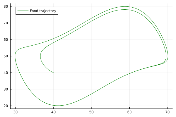

Advanced Visualisations

While we can plot the variables from the ODE component easily, the Agent-based model is a bit more challenging. By default, we only store the variables given in state_names in the solution. This can be changed by providing save_vars=["birds.#model"] to solve, in which case the full agent-based model state will be visible in the solution at all time points.

However, this can be wasteful if we know we only want an animation of the model (which can be generated during simulation). We will set up a Connector which takes an input of the model's current state, and instead of a transformation, we will use a function which adds the current state to a video.

using CairoMakie

const bird_polygon = Makie.Polygon(Point2f[(-1, -1), (2, 0), (-1, 1)])
function bird_marker(b::Bird)
    φ = atan(b.vel[2], b.vel[1]) #+ π/2 + π
    return rotate_polygon(bird_polygon, φ)
end

fig, ax = abmplot(model; agent_marker = bird_marker)
CairoMakie.scatter!(ax, [model.food_x], [model.food_y], markersize = 35, color = :green)
io = VideoStream(fig)
function plot_input(model)
    empty!(ax)
    abmplot!(
        ax, model; agent_marker = bird_marker)
    CairoMakie.scatter!(ax, [model.food_x], [model.food_y], markersize = 35, color = :green)
    recordframe!(io)
end

conn3 = Connector(
    inputs = ["birds.#model"],
    outputs = Vector{String}(),
    func = (model) -> plot_input(model)
)

sp = SirenProblem(components = [comp1, comp2], connectors = [conn1, conn2, conn3], tspan = tspan)
sol = solve(sp, alg)

save("birds.mp4", io)